from sklearn.neural_network import MLPClassifier
import numpy as np다층 퍼셉트론과 딥러닝
딥러닝
퍼셉트론
ref
XOR연산
1. 패키지 설정
2. 데이터 작성
X=np.array([[0,0],[0,1],[1,0],[1,1]])
y=np.array([0,1,1,0])- 입력 값, 목표 값 작성
3. 모형화
model=MLPClassifier(hidden_layer_sizes=(2),
                    activation='logistic',
                    solver='lbfgs',
                    max_iter=100)
4. 학습
model.fit(X,y)MLPClassifier(activation='logistic', hidden_layer_sizes=2, max_iter=100,
solver='lbfgs')In a Jupyter environment, please rerun this cell to show the HTML representation or trust the notebook. On GitHub, the HTML representation is unable to render, please try loading this page with nbviewer.org.
MLPClassifier(activation='logistic', hidden_layer_sizes=2, max_iter=100,
solver='lbfgs')5. 예측
print(model.predict(X))[0 0 1 0]비선형 함수의 회귀분석
1. 패키지 설정
from sklearn.neural_network import MLPRegressor
from sklearn.preprocessing import MinMaxScaler
from sklearn.model_selection import train_test_split
from sklearn.metrics import mean_absolute_percentage_error
import numpy as np
import matplotlib.pyplot as plt
2. 데이터 준비
X=np.array(range(1,101))
print(X)
[ 1 2 3 4 5 6 7 8 9 10 11 12 13 14 15 16 17 18
19 20 21 22 23 24 25 26 27 28 29 30 31 32 33 34 35 36
37 38 39 40 41 42 43 44 45 46 47 48 49 50 51 52 53 54
55 56 57 58 59 60 61 62 63 64 65 66 67 68 69 70 71 72
73 74 75 76 77 78 79 80 81 82 83 84 85 86 87 88 89 90
91 92 93 94 95 96 97 98 99 100]y=0.5*(X-50)**3 - 50000/X + 120000
print(y)[ 11175.5 39704. 51421.83333333 58832.
64437.5 69074.66666667 73103.64285714 76706.
79983.94444444 83000. 85795.04545455 88397.33333333
90827.34615385 93100.57142857 95229.16666667 97223.
99090.32352941 100838.22222222 102472.92105263 104000.
105424.54761905 106751.27272727 107984.58695652 109128.66666667
110187.5 111164.92307692 112064.64814815 112890.28571429
113645.36206897 114333.33333333 114957.59677419 115521.5
116028.34848485 116481.41176471 116883.92857143 117239.11111111
117550.14864865 117820.21052632 118052.44871795 118250.
118415.98780488 118553.52380952 118665.70930233 118755.63636364
118826.38888889 118881.04347826 118922.67021277 118954.33333333
118979.09183673 119000. 119020.10784314 119042.46153846
119070.10377358 119106.07407407 119153.40909091 119215.14285714
119294.30701754 119393.93103448 119517.04237288 119666.66666667
119845.82786885 120057.5483871 120304.84920635 120590.75
120918.26923077 121290.42424242 121710.23134328 122180.70588235
122704.86231884 123285.71428571 123926.27464789 124629.55555556
125398.56849315 126236.32432432 127145.83333333 128130.10526316
129192.14935065 130334.97435897 131561.58860759 132875.
134278.21604938 135774.24390244 137366.09036145 139056.76190476
140849.26470588 142746.60465116 144751.78735632 146867.81818182
149097.70224719 151444.44444444 153911.04945055 156500.52173913
159215.8655914 162060.08510638 165036.18421053 168147.16666667
171396.03608247 174785.79591837 178319.44949495 182000. ]3. 탐색적 데이터 분석
plt.scatter(X, y, color='b')
plt.title('y=0.5*(X-50)**3 - 50000/X + 120000')
plt.xlabel('X')
plt.ylabel('y')
plt.ylim(0,200000)
plt.show()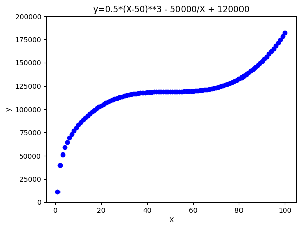
4. 데이터 분리
X_train, X_test, y_train, y_test = train_test_split(X,y, test_size=0.3,
random_state=1234)print(X_train)
print(X_test)[ 5 65 11 94 58 73 37 8 55 78 22 19 71 87 23 7 45 9
42 17 46 21 26 56 79 32 93 6 85 33 53 14 92 18 29 47
61 15 66 13 20 3 4 1 12 68 98 35 38 96 51 100 74 81
70 59 91 90 44 31 27 24 50 16 25 77 54 39 84 48]
[41 36 82 62 99 69 86 28 40 43 34 60 64 95 57 88 97 2 72 83 10 52 30 89
76 75 63 67 80 49]print(y_train)
print(y_test)[ 64437.5 120918.26923077 85795.04545455 162060.08510638
119393.93103448 125398.56849315 117550.14864865 76706.
119153.40909091 130334.97435897 106751.27272727 102472.92105263
123926.27464789 144751.78735632 107984.58695652 73103.64285714
118826.38888889 79983.94444444 118553.52380952 99090.32352941
118881.04347826 105424.54761905 111164.92307692 119215.14285714
131561.58860759 115521.5 159215.8655914 69074.66666667
140849.26470588 116028.34848485 119070.10377358 93100.57142857
156500.52173913 100838.22222222 113645.36206897 118922.67021277
119845.82786885 95229.16666667 121290.42424242 90827.34615385
104000. 51421.83333333 58832. 11175.5
88397.33333333 122180.70588235 174785.79591837 116883.92857143
117820.21052632 168147.16666667 119020.10784314 182000.
126236.32432432 134278.21604938 123285.71428571 119517.04237288
153911.04945055 151444.44444444 118755.63636364 114957.59677419
112064.64814815 109128.66666667 119000. 97223.
110187.5 129192.14935065 119106.07407407 118052.44871795
139056.76190476 118954.33333333]
[118415.98780488 117239.11111111 135774.24390244 120057.5483871
178319.44949495 122704.86231884 142746.60465116 112890.28571429
118250. 118665.70930233 116481.41176471 119666.66666667
120590.75 165036.18421053 119294.30701754 146867.81818182
171396.03608247 39704. 124629.55555556 137366.09036145
83000. 119042.46153846 114333.33333333 149097.70224719
128130.10526316 127145.83333333 120304.84920635 121710.23134328
132875. 118979.09183673]5. 피처 스케일링
X_train = X_train.reshape(-1,1)
X_test=X_test.reshape(-1,1)
y_train=y_train.reshape(-1,1)
y_test=y_test.reshape(-1,1)
print(X_train)
[[ 5]
[ 65]
[ 11]
[ 94]
[ 58]
[ 73]
[ 37]
[ 8]
[ 55]
[ 78]
[ 22]
[ 19]
[ 71]
[ 87]
[ 23]
[ 7]
[ 45]
[ 9]
[ 42]
[ 17]
[ 46]
[ 21]
[ 26]
[ 56]
[ 79]
[ 32]
[ 93]
[ 6]
[ 85]
[ 33]
[ 53]
[ 14]
[ 92]
[ 18]
[ 29]
[ 47]
[ 61]
[ 15]
[ 66]
[ 13]
[ 20]
[ 3]
[ 4]
[ 1]
[ 12]
[ 68]
[ 98]
[ 35]
[ 38]
[ 96]
[ 51]
[100]
[ 74]
[ 81]
[ 70]
[ 59]
[ 91]
[ 90]
[ 44]
[ 31]
[ 27]
[ 24]
[ 50]
[ 16]
[ 25]
[ 77]
[ 54]
[ 39]
[ 84]
[ 48]]scalerX=MinMaxScaler()
scalerX.fit(X_train)
X_train_norm=scalerX.transform(X_train)scalerY=MinMaxScaler()
scalerY.fit(y_train)
y_train_norm=scalerY.transform(y_train)X_test_norm=scalerX.transform(X_test)
y_test_norm=scalerY.transform(y_test)6. 모형화 및 학습
model=MLPRegressor(hidden_layer_sizes=(4),
                   activation='logistic',
                   solver='lbfgs',
max_iter=500)model.fit(X_train_norm,y_train_norm)/home/coco/anaconda3/envs/py38/lib/python3.8/site-packages/sklearn/neural_network/_multilayer_perceptron.py:1623: DataConversionWarning: A column-vector y was passed when a 1d array was expected. Please change the shape of y to (n_samples, ), for example using ravel().
y = column_or_1d(y, warn=True)MLPRegressor(activation='logistic', hidden_layer_sizes=4, max_iter=500,
solver='lbfgs')In a Jupyter environment, please rerun this cell to show the HTML representation or trust the notebook. On GitHub, the HTML representation is unable to render, please try loading this page with nbviewer.org.
MLPRegressor(activation='logistic', hidden_layer_sizes=4, max_iter=500,
solver='lbfgs')7. 예측
y_pred=model.predict(X_test_norm)
print(y_pred)
[0.58532633 0.5596793 0.78666172 0.69076416 0.86381245 0.72489815
0.80520178 0.51832425 0.58021083 0.59553508 0.5493746 0.68090896
0.70057482 0.84605491 0.66604552 0.81438502 0.85496516 0.38241064
0.73934651 0.79131812 0.42434114 0.64106953 0.52869543 0.81895453
0.75843272 0.7536807 0.69567514 0.71520447 0.77730687 0.62596952]# 데이터 구조의 변형
y_pred=y_pred.reshape(-1,1)# 예측 값의 역변환
y_pred_inverse=scalerY.inverse_transform(y_pred)
print(y_pred_inverse)[[111163.57767477]
[106782.43697013]
[145556.59434008]
[129174.94277171]
[158735.82920511]
[135005.86461054]
[148723.69087489]
[ 99717.9814556 ]
[110289.72571243]
[112907.48205149]
[105022.14122011]
[127491.43180009]
[130850.84418785]
[155702.4069167 ]
[124952.39323735]
[150292.41387152]
[157224.4958677 ]
[ 76500.60587199]
[137473.99775244]
[146352.02276425]
[ 83663.3625764 ]
[120685.88219775]
[101489.63200544]
[151072.99795266]
[140734.38957096]
[139922.62822513]
[130013.85862295]
[133349.94535149]
[143958.55773291]
[118106.43080755]]plt.scatter(X,y, color='g')
# 원데이터
plt.title('y=0.5*(X-50)**3 - 50000/X + 120000')
plt.xlabel('X')
plt.ylabel('y')
plt.ylim(0,200000)
# 테스트데이터
plt.scatter(X_test, y_pred_inverse, color='r')
plt.show()
print('MAPE:%.2f' %
      mean_absolute_percentage_error(y_test,y_pred_inverse))
MAPE:0.10